Highly Complex Distributions

What happens when real-world data refuses to behave — and why that’s actually interesting.

When Normal Isn’t Normal

I’ve spent enough time working with real-world datasets to know that they almost never cooperate with the textbook stories we tell about them. A sensor network that should produce clean Gaussian readings? It has periodic glitches. Customer behaviour? It clusters into sub-populations with wildly different patterns. Financial returns? They occasionally spike in ways that break every model you’ve built.

When I first encountered data like this, I made the mistake of forcing it into standard distributions and pretending the fit was “good enough.” It wasn’t. The models I built on top of that assumption failed silently—predictions looked reasonable until they weren’t, and by then the damage was done.

This post explores what happens when distributions refuse to be simple. Not in a theoretical sense, but in a practical one: what does the data actually look like, and why should you care?

A tale of two peaks (and a fat tail)

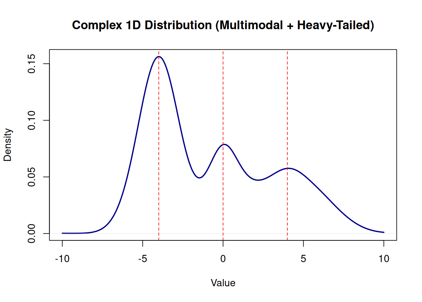
Imagine your data comes not from a single source, but from several invisible sub-populations mixed together. The first group clusters around -4, the second around 4, and then there’s that small but stubborn third group that generates occasional extreme outliers from a distribution so unruly it doesn’t even have a well-defined mean or variance.

This is a mixture distribution—a combination of multiple underlying patterns masquerading as one. The first two components are normal distributions (think of them as “well-behaved”). The third, a Cauchy distribution, is the troublemaker. It’s theoretically centered at 0, but its tails are so heavy that even a tiny percentage from this component can stretch your x-axis to absurd values. The visualization below shows what this looks like when you truncate the axis to a reasonable window—if you expanded it further, you’d see those Cauchy-generated outliers sprawling to the edges of the plot.

Figure 1: 1D Multimodal and Heavy-Tailed Mixture Distribution - Combines standard normal distributions with a heavy-tailed Cauchy distribution.

Now add a second dimension

Real data doesn’t exist in isolation. It lives in multidimensional space—sometimes you’re tracking two variables, sometimes dozens. When you move from one dimension to two or more, things get interesting in ways that 1D intuition doesn’t prepare you for.

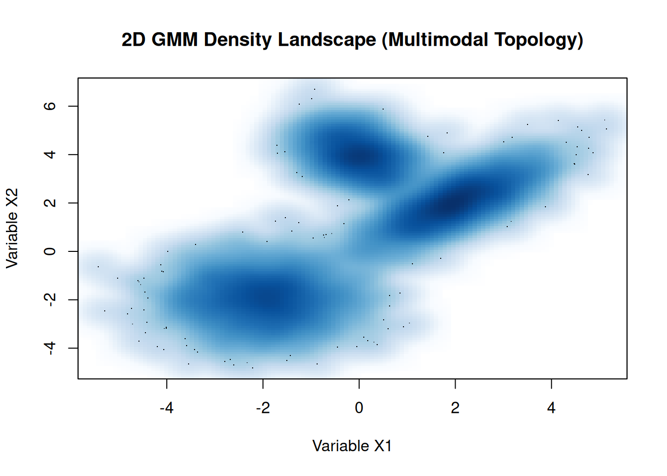
In multi-dimensional mixture models, each sub-population doesn’t just have a different center; it has a different shape. Some clusters might be spherical (equal spread in all directions), while others are elongated (highly correlated across variables) or compressed asymmetrically. These covariance structures matter enormously in practice. If you’re clustering customer behavior or sensor readings, you need a method that recognizes that one segment might form a tight, elongated blob while another spreads out more diffusely.

The plot below shows a 2D Gaussian Mixture Model with three components, each with a distinct covariance structure. The first is spherical, the second shows strong positive correlation (the data points form an elongated diagonal cloud), and the third is compressed and oriented differently. This is the kind of landscape you encounter in genomics, where gene expression patterns cluster differently across tissues, or in user segmentation, where behavioral patterns vary wildly by demographic.

Figure 2: 2D Gaussian Mixture Model (GMM) - Simulates a multi-variable landscape featuring intricate dependencies.

So why does complexity matter?

Here’s the thing: most standard algorithms—k-means clustering, linear regression, even many neural network architectures—were built with implicit assumptions about how data behaves. They assume your data comes from a single, well-behaved distribution. They assume that outliers are rare mistakes rather than a genuine 20% of your data. They assume that the relationship between variables is relatively smooth and linear.

When your data violates these assumptions, the algorithms don’t fail loudly. They fail silently. Your model trains without error messages. Cross-validation scores look fine. But in production, it drifts—sometimes catastrophically. Clustering assignments collapse, predictions become biased, and confidence intervals that looked reasonable on training data don’t hold up.

Multimodality, heavy tails, and intricate covariance structure aren’t mathematical curiosities. They’re the ground truth of real-world data, and they bite you the moment you pretend they don’t exist. Learning to spot them, to simulate them, and to build models that handle them—that’s where the actual work of applied data science begins.