Dimensionality reduction is a key process in machine learning and data science, allowing us to simplify datasets without losing critical information. The technique you choose, however, largely depends on the relationship between features in your dataset, particularly their correlation.
This post will explore the relationship between feature correlation and the dimensionality reduction method to use, using a practical example with the Wine Quality dataset from Kaggle.We’ll explore common techniques like Principal Component Analysis (PCA), t-SNE, and UMAP, applying them based on feature correlations and discussing when each method works best.
Why Feature Correlation Matters
Highly correlated features tend to carry redundant information, which can bloat a model without improving accuracy. In this case, methods like PCA are effective at reducing redundancy.
Uncorrelated features might not benefit from linear methods like PCA. In such scenarios, non-linear techniques like t-SNE or UMAP can reveal more meaningful structures. The relationship between features guides our choice of dimensionality reduction methods, helping us retain the most relevant information in the data.
The Wine Quality dataset which we will use from Kaggle contains physical and chemical properties of wines (like acidity, sugar levels, and alcohol content) and a target variable, quality, which rates the wine on a scale from 0 to 10. The dataset is simple enough for us to explore how to reduce dimensionality based on feature correlation.
Explorative Analysis
Inspecting the Dataset
The dataset summary is
summary(wine_data)
##  fixed.acidity    volatile.acidity  citric.acid     residual.sugar
##  Min.   : 4.600   Min.   :0.1200   Min.   :0.0000   Min.   : 0.900
##  1st Qu.: 7.100   1st Qu.:0.3925   1st Qu.:0.0900   1st Qu.: 1.900
##  Median : 7.900   Median :0.5200   Median :0.2500   Median : 2.200
##  Mean   : 8.311   Mean   :0.5313   Mean   :0.2684   Mean   : 2.532
##  3rd Qu.: 9.100   3rd Qu.:0.6400   3rd Qu.:0.4200   3rd Qu.: 2.600
##  Max.   :15.900   Max.   :1.5800   Max.   :1.0000   Max.   :15.500
##    chlorides       free.sulfur.dioxide total.sulfur.dioxide    density
##  Min.   :0.01200   Min.   : 1.00       Min.   :  6.00       Min.   :0.9901
##  1st Qu.:0.07000   1st Qu.: 7.00       1st Qu.: 21.00       1st Qu.:0.9956
##  Median :0.07900   Median :13.00       Median : 37.00       Median :0.9967
##  Mean   :0.08693   Mean   :15.62       Mean   : 45.91       Mean   :0.9967
##  3rd Qu.:0.09000   3rd Qu.:21.00       3rd Qu.: 61.00       3rd Qu.:0.9978
##  Max.   :0.61100   Max.   :68.00       Max.   :289.00       Max.   :1.0037
##        pH          sulphates         alcohol         quality
##  Min.   :2.740   Min.   :0.3300   Min.   : 8.40   Min.   :3.000
##  1st Qu.:3.205   1st Qu.:0.5500   1st Qu.: 9.50   1st Qu.:5.000
##  Median :3.310   Median :0.6200   Median :10.20   Median :6.000
##  Mean   :3.311   Mean   :0.6577   Mean   :10.44   Mean   :5.657
##  3rd Qu.:3.400   3rd Qu.:0.7300   3rd Qu.:11.10   3rd Qu.:6.000
##  Max.   :4.010   Max.   :2.0000   Max.   :14.90   Max.   :8.000
##        Id
##  Min.   :   0
##  1st Qu.: 411
##  Median : 794
##  Mean   : 805
##  3rd Qu.:1210
##  Max.   :1597
Diving a little deeper, lets also look at the extended dataset summary
Table: Table 1: Data summary
| Name | wine_data |
| Number of rows | 1143 |
| Number of columns | 13 |
| _______________________ | |
| Column type frequency: | |
| numeric | 13 |
| ________________________ | |
| Group variables | None |
Variable type: numeric
| skim_variable | n_missing | complete_rate | mean | sd | p0 | p25 | p50 | p75 | p100 | hist |
|---|---|---|---|---|---|---|---|---|---|---|
| fixed.acidity | 0 | 1 | 8.31 | 1.75 | 4.60 | 7.10 | 7.90 | 9.10 | 15.90 | ▂▇▂▁▁ |
| volatile.acidity | 0 | 1 | 0.53 | 0.18 | 0.12 | 0.39 | 0.52 | 0.64 | 1.58 | ▅▇▂▁▁ |
| citric.acid | 0 | 1 | 0.27 | 0.20 | 0.00 | 0.09 | 0.25 | 0.42 | 1.00 | ▇▆▅▁▁ |
| residual.sugar | 0 | 1 | 2.53 | 1.36 | 0.90 | 1.90 | 2.20 | 2.60 | 15.50 | ▇▁▁▁▁ |
| chlorides | 0 | 1 | 0.09 | 0.05 | 0.01 | 0.07 | 0.08 | 0.09 | 0.61 | ▇▁▁▁▁ |
| free.sulfur.dioxide | 0 | 1 | 15.62 | 10.25 | 1.00 | 7.00 | 13.00 | 21.00 | 68.00 | ▇▅▂▁▁ |
| total.sulfur.dioxide | 0 | 1 | 45.91 | 32.78 | 6.00 | 21.00 | 37.00 | 61.00 | 289.00 | ▇▂▁▁▁ |
| density | 0 | 1 | 1.00 | 0.00 | 0.99 | 1.00 | 1.00 | 1.00 | 1.00 | ▁▃▇▂▁ |
| pH | 0 | 1 | 3.31 | 0.16 | 2.74 | 3.20 | 3.31 | 3.40 | 4.01 | ▁▅▇▂▁ |
| sulphates | 0 | 1 | 0.66 | 0.17 | 0.33 | 0.55 | 0.62 | 0.73 | 2.00 | ▇▅▁▁▁ |
| alcohol | 0 | 1 | 10.44 | 1.08 | 8.40 | 9.50 | 10.20 | 11.10 | 14.90 | ▇▇▃▁▁ |
| quality | 0 | 1 | 5.66 | 0.81 | 3.00 | 5.00 | 6.00 | 6.00 | 8.00 | ▁▇▇▂▁ |
| Id | 0 | 1 | 804.97 | 464.00 | 0.00 | 411.00 | 794.00 | 1209.50 | 1597.00 | ▇▇▇▇▇ |
The important factors to look for is n_missing for each feature.
Missing data can adversely impact correlation calculations. In our
dataset, we do not have any missing values.
The mean and sd gives you a sense of centrality and dispersion for
each feature. In our case, we can see that volatile acidity, citric
acid, chlorides, density, suphates and density have the lowest standard
deviations and so have very low spread. A low SD means the data is more
predictable since it tends to stay close to the average.
The dataset has 12 features (such as acidity, sugar levels, and pH) and one target column (wine quality). Our goal is to reduce the dimensionality of the features while maintaining enough information to distinguish between different quality ratings.
Correlation Analysis
First lets look at the correlation p-values, taking only the first 4 variables to show how the results can be interpretted
| fixed.acidity | volatile.acidity | citric.acid | residual.sugar | |
|---|---|---|---|---|
| fixed.acidity | 0.0000000 | 0.0000000 | 0.0000000 | 0.0000000 |
| volatile.acidity | 0.0000000 | 0.0000000 | 0.0000000 | 0.8460008 |
| citric.acid | 0.0000000 | 0.0000000 | 0.0000000 | 0.0000000 |
| residual.sugar | 0.0000000 | 0.8460008 | 0.0000000 | 0.0000000 |
| chlorides | 0.0002580 | 0.0569023 | 0.0000000 | 0.0165682 |
| free.sulfur.dioxide | 0.0000000 | 0.9471585 | 0.0515978 | 0.0000000 |
| total.sulfur.dioxide | 0.0001786 | 0.0085480 | 0.2129081 | 0.0000000 |
| density | 0.0000000 | 0.5770811 | 0.0000000 | 0.0000000 |
| pH | 0.0000000 | 0.0000000 | 0.0000000 | 0.0000739 |
| sulphates | 0.0000000 | 0.0000000 | 0.0000000 | 0.5550689 |
| alcohol | 0.0111399 | 0.0000000 | 0.0003202 | 0.0483106 |
Lower p-values indicates the correlation to be significant, a value of 0 indicates perfect correlation. Plotting it makes the information more apparent.
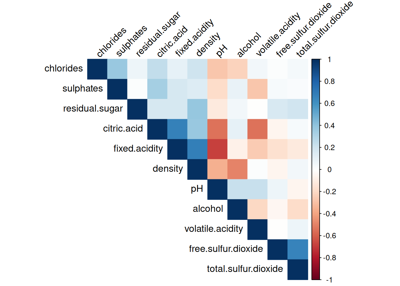
Observations:
Strong correlations exist between some features, such as total sulfur dioxide and free sulfur dioxide, and density and residual sugar. Other features, such as citric acid and pH, show weaker correlations with the rest of the data.
This analysis shows that Principal Component Analysis (PCA) might be useful for removing redundancy, while non-linear methods may reveal deeper relationships.
Dimensionality Reduction
Principal Component Analysis
PCA is ideal for datasets where features are highly correlated. It projects correlated features into a set of orthogonal (uncorrelated) components, ordered by the amount of variance they explain.
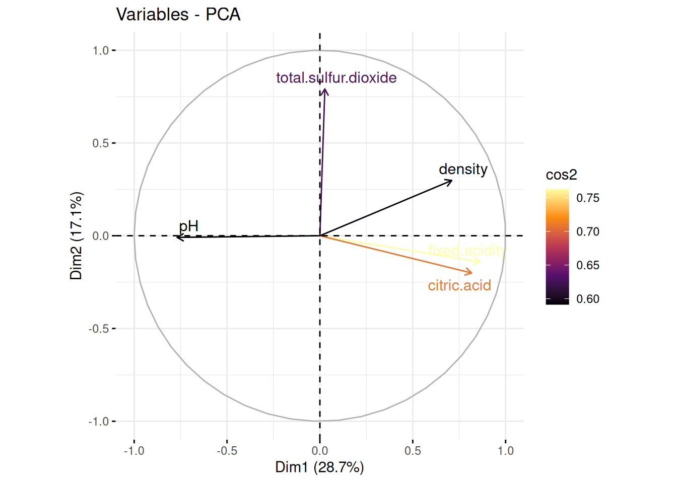
Now, lets look at the top 5 contributing variables.
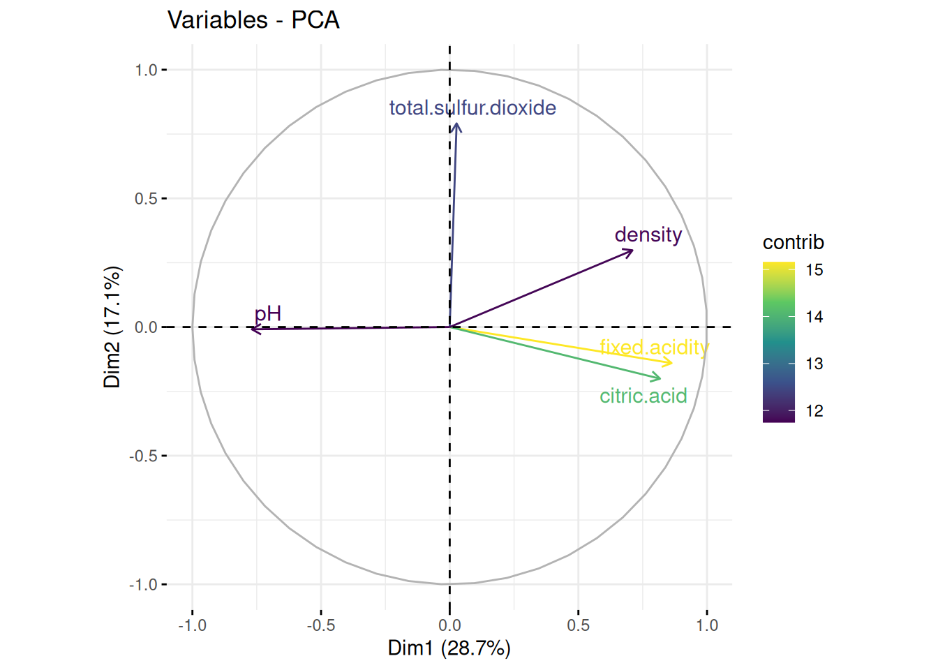
pH is negatively correlated with Dim1, density is positively correlated with both Dim1 and Dim2, acidity (fixed acidity and citric acid) is positively correlated with Dim1 but slightly negatively correlated with Dim2. Total Sulphur Dioxide is positively correlated with Dim2 but very slightly positively correlated with Dim1
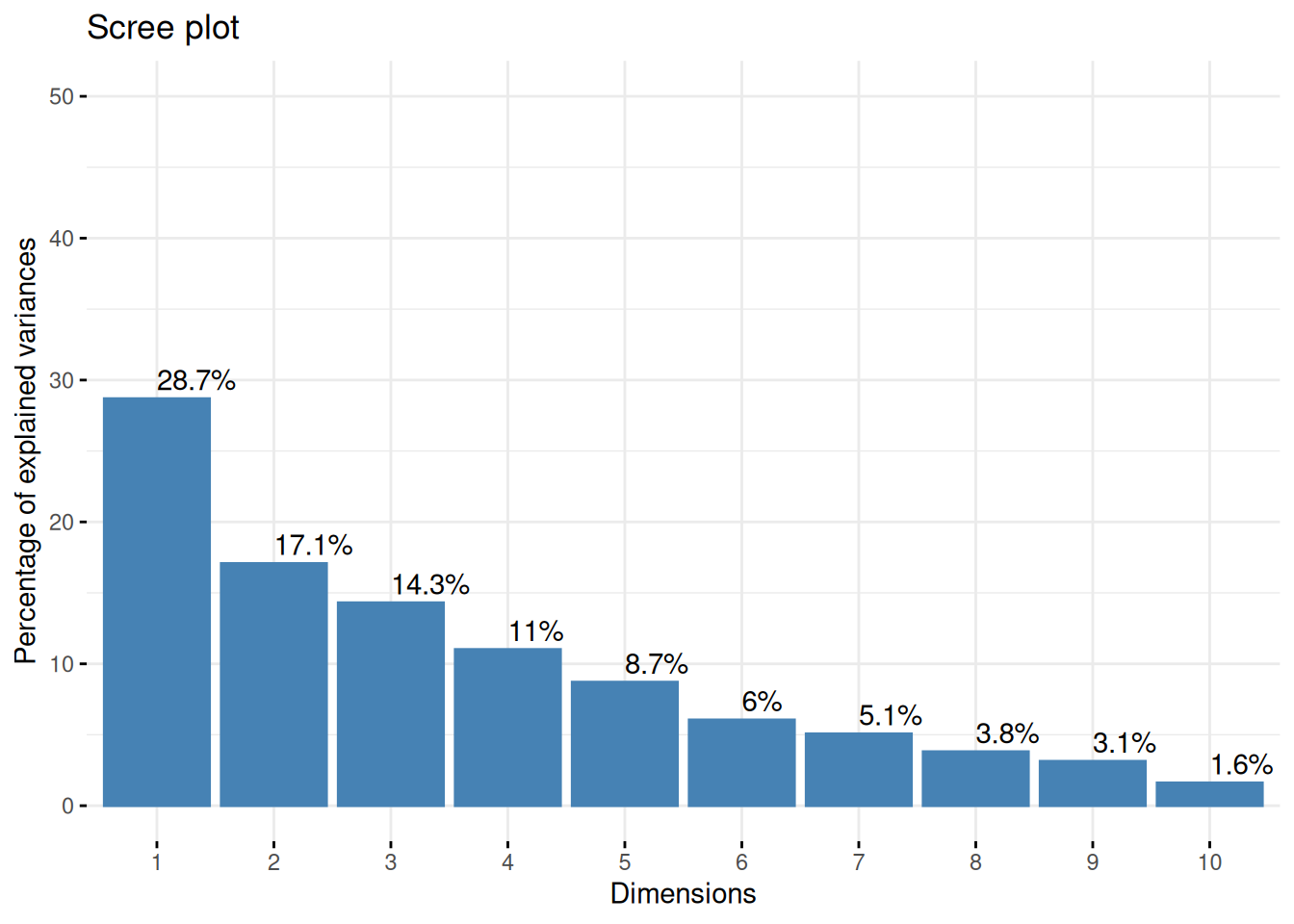
Please keep in mind that Dim1 explains 28.7% of the variances and Dim2 explains 17.1% of the variances.
Observations
-
Dim1 (28.7% of the variance): This dimension explains the largest portion of the variance in the data. Since pH is negatively correlated with Dim1, while density is positively correlated, Dim1 likely represents a contrast between wines with high pH and those with high density.
-
Dim2 (17.1% of the variance): This dimension explains a smaller, but still substantial, portion of the variance. Density is positively correlated, Acidity is negatively correlated approximate to the same extent . Dim2 could represent a different axis of variation that distinguishes wines based on acidity and density. Total Suphur dioxide is very positively correlated with this dimension.
While Dim1 is more heavily influenced by factors like pH and density, Dim2 seems to capture a dimension of variation more closely related to preservation techniques and perhaps chemical stability in wine.
t-SNE for Non-Linear Relationships
This is applied for Low or Non-correlated Features since PCA is linear and does not work well for non linear relationships. The features which are correlated and have linear relationships are removed from the dataset so that they do not overshadow the results.
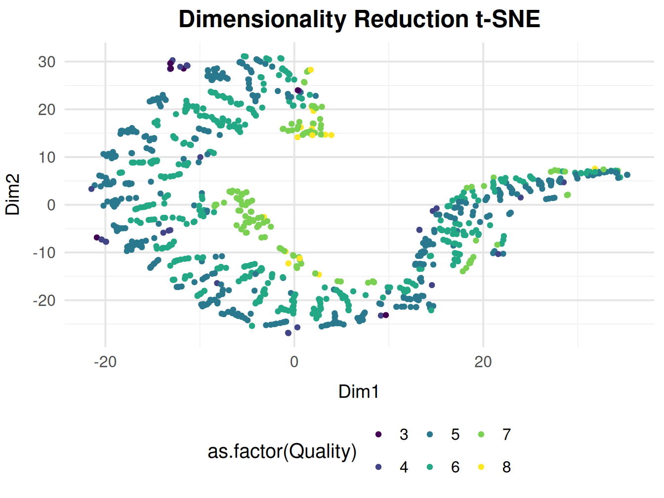
t-SNE is complete, the result set is as below after adding the quality and quality grade for better analysis
Let’s check how this dataset looks like
head(tsne_data, 10)
##          Dim1       Dim2 Quality Quality.Grade
## 1  -18.738882  -4.753947       5        Medium
## 2   14.263076  -7.654165       5        Medium
## 3   -8.436640 -19.917958       5        Medium
## 4   -1.341963 -21.843421       6        Medium
## 5  -15.140696 -12.933188       5        Medium
## 6   -9.637007 -20.807349       5        Medium
## 7   -1.546742  -9.081253       7          High
## 8   -6.533065   2.946497       7          High
## 9   -9.439908 -20.998677       5        Medium
## 10  -6.474126 -21.987827       5        Medium
Plotting Using Quality
Plotting Using Quality Grade
Categorising using grades will yield greater clarity of how the quality is distributed acoross the dimensions
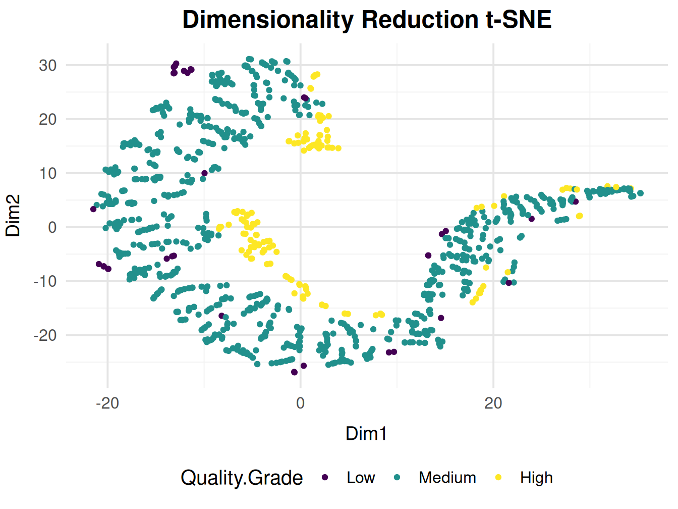
Obvervations
Since we removed the features correlated with principal components in PCA (such as pH, density, acidity (total + citric acid), and sulfur dioxide) to focus on other variables. The t-SNE plot now shows clusters that reflect the remaining features. This suggests that the wine quality is influenced by variables other than those captured in the original PCA.
Since t-SNE emphasizes local relationships, the wines in this cluster are likely more similar to each other based on the remaining features (after correlated features were removed).
t-SNE often uncovers non-linear relationships that PCA might miss. The highest quality wines in this cluster could be influenced by complex, multi-dimensional interactions between the remaining features, which were not linearly separable in PCA but are captured by t-SNE.
The observations based on our visualization remain inconclusive for this dimensionality reduction method.
UMAP for Better Global Structure
While t-SNE focuses on local structure, UMAP (Uniform Manifold Approximation and Projection) can preserve both local and global structure in the data. It’s also faster than t-SNE, making it a popular choice for large datasets.
So that the clusters are clearly visible in terms of quality, I am now categorizing the quality into low, medium and high.
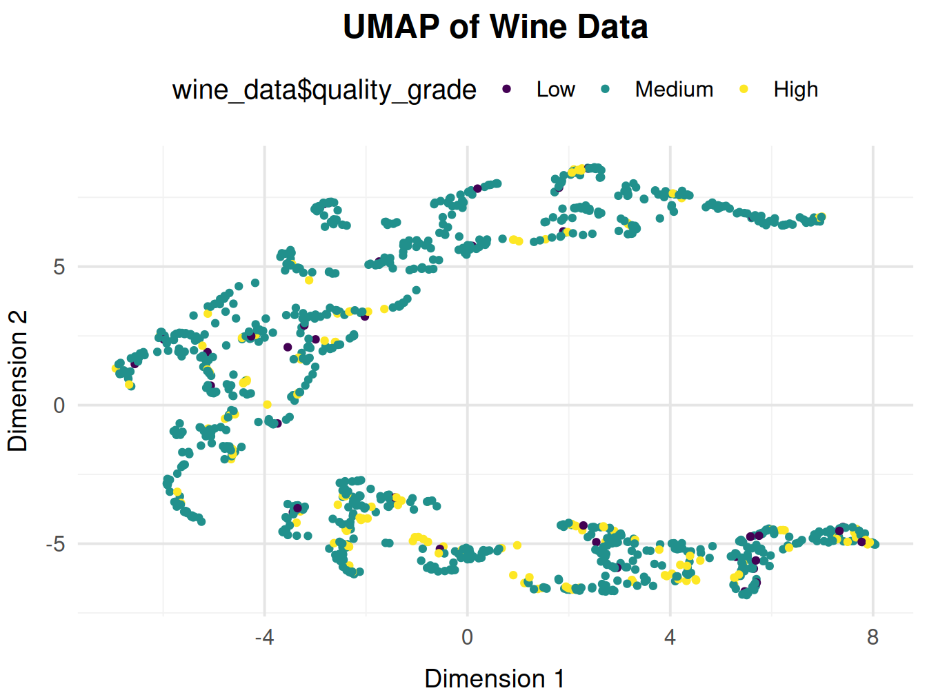
Good quality wines seem to be positively correlated with Dim1 and negatively correlated with Dim2. So lets look a little deeper into the relationship between the original variables and UMAP dimensions
Visualize or inspect correlations
cor_dim1
##                             [,1]
## fixed.acidity         0.02995035
## volatile.acidity     -0.46090659
## citric.acid           0.19612588
## residual.sugar       -0.15341425
## chlorides            -0.23784499
## free.sulfur.dioxide  -0.12172277
## total.sulfur.dioxide -0.37514193
## density              -0.36093523
## pH                    0.14289373
## sulphates             0.19282060
## alcohol               0.69083989
## quality               0.69115710
## Dim1                  1.00000000
## Dim2                 -0.21397845
cor_dim2
##                             [,1]
## fixed.acidity        -0.74725288
## volatile.acidity      0.52343047
## citric.acid          -0.82743197
## residual.sugar       -0.21929042
## chlorides            -0.28564198
## free.sulfur.dioxide   0.12730819
## total.sulfur.dioxide  0.01770915
## density              -0.43451184
## pH                    0.66907273
## sulphates            -0.40096727
## alcohol              -0.05876562
## quality              -0.30047988
## Dim1                 -0.21397845
## Dim2                  1.00000000
This will give us the correlations of each variable with Dim1 and Dim2. You
can interpret the following:
-
Positive correlations with Dim1: Variables that increase as Dim1 increases contribute positively to Dim1. The variables like fixed.acidity, citric.acid, pH (very low correlation), sulphates, quality and alcohol fall into this category.
-
Negative correlations with Dim2: Variables that increase as Dim2 decreases contribute negatively to Dim2. Variables like volatile.acidity, free and total sufurdioxide, pH (very high correlation) fall into this category.
From the data, Dim1 seems to be positively correlated to the quality of the wine and Dim2 seems to be negatively correlated with the quality of wine.
Summarizing the Analysis
In real-world wine analysis, the quality of a wine can be related to several chemical properties. Principal Component Analysis (PCA) and Uniform Manifold Approximation and Projection (UMAP) can help identify key factors influencing wine quality.
- Insights from PCA:
Dim1 (28.7% variance): Represents the largest variation in the data and highlights a contrast between wines with high pH (low acidity) and wines with higher density. This suggests that wines with higher density (which could be linked to richer flavors or higher sugar/alcohol content) are generally of better quality than those with higher pH, which can sometimes indicate flatter wines.
Dim2 (17.1% variance): Reflects a different set of factors, primarily involving acidity and chemical stability (e.g., total sulfur dioxide used for preservation). Wines with higher acidity tend to be better in quality, while higher sulfur dioxide may be indicative of lower quality, as it is often used to preserve wines that might be less stable naturally.
- Insights from UMAP:
Positive correlation with Dim1:
Factors like fixed acidity, citric acid, alcohol, and sulphates correlate positively with wine quality. Higher acidity and alcohol content often signal a well-balanced, higher-quality wine.
Negative correlation with Dim2:
Factors like volatile acidity, sulfur dioxide levels, and pH are negatively correlated. High volatile acidity and sulfur dioxide indicate wines that may have preservation issues or chemical instability, often suggesting lower quality.
Conclusion
By applying PCA and UMAP to wine data, we gain valuable insights into the relationships between different chemical properties and wine quality, and how dimensionality reduction helps simplify these complex correlations.
PCA revealed two key dimensions, Dim1, which is primarily driven by density and negatively impacted by pH, and Dim2, influenced by acidity and chemical stability (like sulfur dioxide levels). These dimensions help us understand the trade-offs between richer, denser wines with higher quality and wines that may require more preservation techniques or have less favorable acidity.
UMAP further refined these relationships, showing that variables like fixed acidity , alcohol, and sulphates positively correlate with wine quality, while volatile acidity and sulfur dioxide are negatively correlated. UMAP helps visualize how certain factors—those that enhance flavor, structure, and balance—are aligned with higher quality, while other elements that contribute to instability or overuse of preservatives indicate lower quality.
In summary, dimensionality reduction techniques like PCA and UMAP allow us to untangle the correlations between wine features and their impact on quality. They help distill complex data into meaningful dimensions, making it easier to understand how acidity, density, alcohol content, and preservation techniques shape the overall perception of wine quality. This analysis emphasizes that quality wines strike a delicate balance across these key factors.